How To Run CoDEx
In this tutorial, we present the available functions for calculating Wilson Coefficients (WCs) for a given BSM Lagrangian and describe the necessary workflow to do that. Following functions are mainly used for the bulk of this job:
| treeOutput | Calculates tree level Wilson Coefficients. |
| loopOutput | Calculates 1 loop level Wilson Coefficients. |
| codexOutput | Generic function for WCs calculation upto 1 loop. |
Building the Lagrangian
The Example Model: Electroweak Real Triplet Scalar
Let us demonstrate this with a toy example where the Lagrangian is given in its traditional form:
![]() is the heavy field which is going to be integrated out.
is the heavy field which is going to be integrated out. ![]() is the Standard Model (SM) Higgs.
is the Standard Model (SM) Higgs. ![]() is the mass of
is the mass of ![]() .
. ![]() is the covariant derivative.
is the covariant derivative. ![]() and
and ![]() are the couplings. (
are the couplings. (![]() is internally defined in CoDEx)
is internally defined in CoDEx)
To write the effective Lagrangian for ![]() , we do not need the kinetic terms. We only need the interaction terms e.g. self interaction terms for SM, SM-heavy field interaction, heavy-heavy (different multiplet) interaction terms in the Lagrangian, which we will henceforth refer as 'LBSM'. So, now the reduced structure is
, we do not need the kinetic terms. We only need the interaction terms e.g. self interaction terms for SM, SM-heavy field interaction, heavy-heavy (different multiplet) interaction terms in the Lagrangian, which we will henceforth refer as 'LBSM'. So, now the reduced structure is
We want to adapt this BSM Lagrangian in our notebook file.
Defining the Heavy Fields
CoDEx takes the user-provided information about the heavy fields in a specific format. User needs to create a List, each element of which is again a List representing one heavy field. These sub-lists are each 7 entries long, each of which denote one property of the heavy field.
fieldList = { field1, field2, ⋯ };
field = { fieldName, components, colorDim, isoDim, hyperCharge, spin, mass }
| fieldName | name of the heavy field, used as the head of the Array representing the field. |
| components | number of components in the heavy field. |
| colorDim | dimensionality of the heavy field under SU(3)C |
| isoDim | dimensionality of the heavy field under SU(2)L |
| hyperCharge | hyper-charge of the heavy field under U(1)Y. |
| spin | spin quantum number of the heavy field. |
| mass | variable name representing the mass of the heavy field |
Description of the entries for each field while constructing the field list.
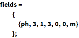
Thus, the whole field list looks like this:
fieldList =
{
{ fieldName1, components1, colorDim1, isoDim1, hyperCharge1, spin1, mass1},
{ fieldName2, components2, colorDim2, isoDim2, hyperCharge2, spin2, mass2},
⋮
⋮
 };
In the case of our example model, we have only one heavy field, a real triplet scalar (i.e. no. of components 3, dimensionality under SU(3)C 1, dimensionality under SU(2)L 3, hyper-charge 0, spin 0). Let us denote the name of the field as 'ph' and its mass as 'm'.
Writing the Lagrangian
Now that our field definitions are ready, it's time to write the Lagrangian in a form that our code understands. For that, first we have to create the representations of these fields in their component form. This is done by a function called 'defineHeavyFields'. Please go to this page for details on how it works.
This can be now written as: - η abs[H]2*Φ.Φ, or - η abs[H]2*abs[Φ]2.
Similarly, the second term can be written as: 2 κ*Table[(dag[H].tau[a].H), {a, 3}].Φ.
And, the third term: -(1/4) λ (Φ.Φ)^2.
LBSM can now be used to find the Wilson Coefficients.
Wilson Coefficients in SMEFT
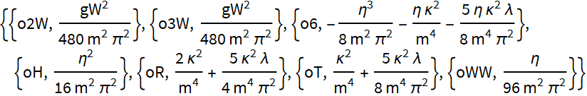
At tree level
This function calculates the tree level Wilson Coefficients for the given Lagrangian in a given operator basis:
| Option Name | Default Value | Details |
| monitor | True | Shows an animation while computing |
| appearance | "Percolate" (for Version ≥11.0) | Appearence of the animation. |
| operBasis | "Warsaw" | Choice of basis of the Dim.-6 operators |
| format | "List" | The output format. |
Options for treeOutput.
The OptionValue selecting the basis of dimension six operators (Option: operBasis) has its default value set to "Warsaw". We can also choose the "SILH" operator basis. Details of these bases are listed in the guide "Operator Bases".
Initializing the model for calculation up to 1 loop
Unlike the tree level case, to calculate 1 loop level WCs, we need the transformation property of the heavy fields under the given gauge symmetry. More precisely, we must know the structure of Isospin and Color symmetry generators determined by the dimensionality of the heavy field’s representations. These are defined by running the function initializeLoop (click on the function name for options and further details).
In the first argument, you provide a name of the model as a string. This will be used to uniquely define the symmetry generators. (here: "ewrts")
In the second argument, you provide list of heavy field definitions ('fields', in this case). The symmetry generators are defined using the information about the Isospin and Color charges for each heavy field from the list of field definitions.
We have provided their structure of representations up to fundamental and quadruplet for SU(3)c and SU(2)L gauge groups respectively. For more exotic BSM particle we have kept provision for one to define it. In that case, you have to define them yourself (you will be prompted to do so in such a case).
For the unlikely case of heavy fields with color dimensionality 6 or more than that, you have to define them yourself (you will be prompted to do so in such a case).
Check the documentation page CoDExParafernalia for details.
All symmetry generators provided by CoDEx are listed in the section 'Symmetry Generators' of the guide 'CoDExParafernalia'.
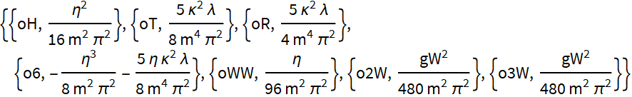
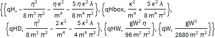
Wilson Coefficients at 1 loop level
| Option Name | Default Value | Details |
| monitor | True | Shows an animation while computing |
| appearance | "Percolate" (for Version ≥11.0) | Appearence of the animation. |
| operBasis | "Warsaw" | Choice of basis of the Dim.-6 operators |
| format | "List" | The output format. |
| style | Large | The fontsize of the output. |
| ibp | True | Turns the 'Integration by Parts' option on. Detail available on the loopOutput page. |
Options for loopOutput.
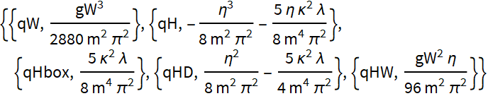
You can see that this takes the model name used by initializeLoop function above (here: "ewrts") to correctly identify the symmetry generators, in addition to the Lagrangian and the list of heavy field definitions. This functionality lets you define multiple models, Lagrangians, and heavy field definitions in the same Notebook and run them without mixing the definitions.
The OptionValue selecting the basis of dimension six operators (Option: operBasis) has its default value set to "Warsaw". We can also choose the "SILH" operator basis. Details of these bases are listed in the guide "Operator Bases".
Using codexOutput: A Single function for everything
codexOutput is a generic function for WCs calculation. Among other options, the tree level or the loop level result can be chosen by changing the option 'outRange'.
| Option Name | Default Value | Details |
| monitor | True | Shows an animation while computing |
| appearance | "Percolate" (for Version ≥11.0) | Appearence of the animation. |
| operBasis | "Warsaw" | Choice of basis of the Dim.-6 operators |
| format | "List" | The output format. |
| model | "" | Takes the same input as initializeLoop. If left blank, will give the tree-level. |
| outRange | "All" | This determines the level at which output is evaluated. 'All' means the result calculates both tree and loop level results and combines them. |
| style | Large | The fontsize of the output. |
| ibp | True | Turns the 'Integration by Parts' option on. Detail available on the loopOutput page. |
Options for codexOutput.
To run this, we again need to run the function initializeLoop. As we have done that above, here can safely run codexOutput. We also need to specify the name of the model that was used in initializeLoop, as the OptionValue of the option 'model'. Failing to do this will give the tree level result, even if the option 'outRange' is set to "Loop" / "All".

- Note! ▶ The OptionValue of the option ' model ' should match with the model name defined in initializeLoop . Otherwise errors will occur.
Details on the output formatting, copying the result in Latex format, and the renormalization group evolution of these Wilson Coefficients can be found in these pages: formPick, texTable and RGFlow.